
One of the most basic machine learning techniques is simple linear regression. In this post I will cover how to implement simple linear regression in Python.
A regression problem is one where you try and predict a target value given one or more features. But let’s break this down a little further, to get a better understanding.
Features
A feature is an individual property or characteristic of the object we’re observing. In short, it can be either a nominal or categorical value. Specifically for simple linear regression all features must be numerical values.
Features are reference by various names, independent variable, predictors, covariates and in algorithms often represented by a upper case X.
| Hours Studied (X) | Grade (y) |
| 10 | 30 |
| 20 | 60 |
| 40 | 80 |
Target
A target is the value you’re trying to predict with a model. It can be either nominal or categorical value but is often represented numerically in both cases.
Target variables are also referenced by various names, such as dependent variable, target variable or as a lower case y in algorithms.
In the case of simple linear regression, our target values will be nominal values.
Origins of Regression
Simple linear regression is not a new concept has been around from the early 1800s. The first published papers were from 1805 and 1806. In both instances regression algorithms were applied to the field of astronomy.
The linear regression method suggests that there is a linear relationship between the independent and dependent variable. Therefore, when the independent variable increases or decreases it has a direct impact on the dependent variable.
Building a Simple Linear Regression model in Python
I believe the best way to learn how something works is to reverse engineer it. This is precisely what I will be covering in this section.
Building your own simple linear regression model in Python is straight forward, however I don’t recommend doing so for any production workloads. There are some very good machine learning libraries which you should use instead. I will show an example using Scikit learn at the end of this article.
Simple Linear Regression Algorithm
The first algorithm you will need to understand is the equation of a straight line. It’s represented as follows:
\large{y = mx + b}
y = how far up the line is drawn in the y axis
x = how far along the x axis
m = slope or gradient of the line
b = value of y when x=0 (starting point)
If you need a refresher on how this is calculated, I’ve found a great article which explains this in detail.
Following on from the equation of a line, the simple linear algorithm is very similar.
\large{y = \beta_0 + \beta_1 x_i}
y = target variable (prediction)
\beta_0 = intercept
\beta_1 = slope
x_i = observation data
It’s relatively straight forward turning the algorithm to Python code. For example, I have written a simple class that implements the algorithm below.
Implementing the algorithm in object orientated programming
import matplotlib.pyplot as plt
import numpy as np
from sklearn.datasets import make_regression
from scipy.stats import norm


class SimpleLinearModel(object):
    def __init__(self):
        self.X = None
        self.y = None
        self.xbar = None
        self.ybar = None
        self.b0 = None
        self.b1 = None

    def fit(self, features: np.array, target: np.array):
        """
        fit the linear model
        :param features: features
        :param target: target
        :return:
        """
        self.X = features
        self.y = target

        self.xbar = np.mean(self.X)
        self.ybar = np.mean(self.y)

        self._covariance()
        self._variance()

    def _covariance(self) -> None:
        """ calculate covariance """
        self.b1 = np.sum((self.X - self.xbar) * (self.y - self.ybar)) / np.sum(np.power(self.X - self.xbar, 2))

    def _variance(self) -> None:
        """ calculate variance """
        self.b0 = self.ybar - (self.b1 * self.xbar)
The class above doesn’t have a predict method, I will cover this shortly.
Creating a simple linear model class
Firstly, the class is initialized with zero values for the required components. Strictly speaking, this isn’t required but it is good practice.
class SimpleLinearModel(object):
    def __init__(self):
        self.X = None
        self.y = None
        self.xbar = None
        self.ybar = None
        self.b0 = None
        self.b1 = None
The fit method
Next we define the fit function, this function essentially calls the two functions that do all the work.
    def fit(self, features: np.array, target: np.array):
        """
        fit the linear model
        :param features: features
        :param target: target
        :return:
        """
        self.X = features
        self.y = target

        self.xbar = np.mean(self.X)
        self.ybar = np.mean(self.y)

        self._covariance()
        self._variance()
Most of the heavily lifting is done by the _covariance and _variance functions. The regression coefficients are calculated here.
Covariance method
Following on is the _covariance function, this is where most of the work is done.
    def _covariance(self) -> None:
        """ calculate covariance """
        self.b1 = np.sum((self.X - self.xbar) * (self.y - self.ybar)) / np.sum(np.power(self.X - self.xbar, 2))
The covariance function implements the covariance method from statistics. Its represented by the following formula.
\Large{ cov_{x,y} = \frac{\sum (x_i - \bar{x})(y_i - \bar{y})}{n - 1} }
x_i = a sample of feature values
y_i = a sample of target values
\bar{x} = the mean of x
\bar{y} = the mean of y
We now have the b1 value or the slope coefficient. Thankfully, numpy takes care of all the matrix math.
Variance method
Lastly, the variance method calculates the intercept value.
    def _variance(self) -> None:
        """ calculate variance """
        self.b0 = self.ybar - (self.b1 * self.xbar)
The formula for variance is:
\Large{ v = \bar{y} - (b_1 * \bar{x})}
\bar{x} = the mean of the sample feature values
\bar{y} = the mean of the sample target values
b_1 = covariance (slope coefficient)
Essentially, we have no covered the basics of the simple linear regression algorithm. But, in order to determine if we have a good fit, we will need some metrics.
Predictions and plotting metrics
Since we’ve got our coefficients, making new predictions on previously unseen data is trivial.
Most importantly, I also included the squared errors and r squared methods which is the most common way to determine fitness of the regression line.
def predict(self, features) -> np.array:
""" predict regression line using exiting model """
return self.b0 + self.b1 * features
@staticmethod
def _squared_error(y, yhat) -> np.array:
""" calculate squared error """
return sum((yhat - y)**2)
def _r_squared(self, y, yhat) -> float:
""" calculate coefficient of determination """
y_mean = np.mean(y)
y_line = [y_mean for _ in y]
se_yhat = self._squared_error(y, yhat)
se_y_mean = self._squared_error(y, y_line)
return 1 - (se_yhat / se_y_mean)
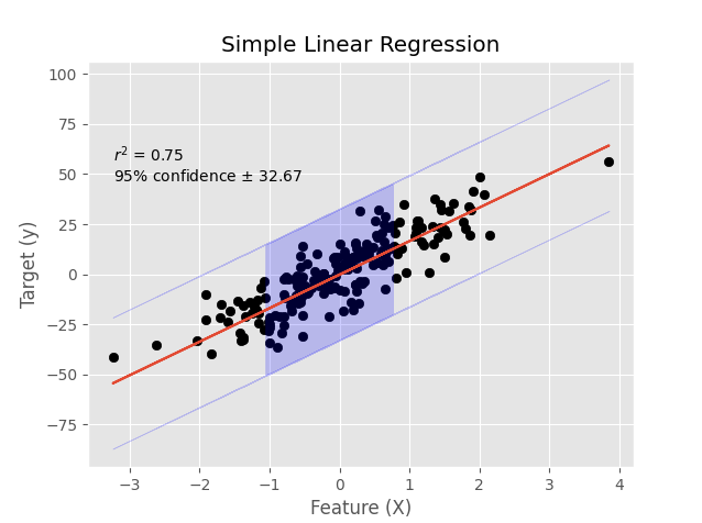
def plot(self, X, y, yhat) -> None:
""" plot regression line """
plt.style.use('ggplot')
r2 = self._r_squared(y, yhat)
conf = norm.interval(0.95, loc=np.mean(yhat), scale=yhat.std())
plt.scatter(X, y, color='black') # actual values
plt.plot(X, yhat) # regression line
plt.fill_between(X.reshape(-1), (yhat+conf[0]), (yhat+conf[1]), color='b', alpha=0.2)
# Labels
plt.text(X.min().min(), y.max().max(), '$r^{2}$ = %s' % round(r2, 2)) # r squared
plt.text(X.min().min(), y.max().max()-10, '95% confidence $\pm$ {:.2f}'.format(abs(conf[0]))) # r squared
plt.title('Simple Linear Regression')
plt.ylabel('Target (y)')
plt.xlabel('Feature (X)')
plt.show()Lastly, the plot method creates a nice graph showing the regression line with a 95% confidence interval. Thanks to the stats package from Scipy, it is very straight forward to do.
For the complete working example have a look at the simple_lr.py on my github.
How should you use linear regression?
As mentioned earlier in this post, I will also show you how to implement the same concept with a tried and tested library.
My library of choice when it comes to machine learning is sci-kit learn. What we’ve covered in this post can be achieved much more concisely with sci-kit learn.
Below will give you the same results as above, a full working example can be seen here – simple_lr_sklearn.py.
import matplotlib.pyplot as plt
from sklearn.datasets import make_regression
from sklearn.linear_model import LinearRegression
from sklearn.model_selection import train_test_split

from plot_functions import plot_regression


if __name__ == '__main__':

    # generate regression dataset
    n_samples = 1000
    X, y = make_regression(n_samples=1000, n_features=1, n_targets=1, random_state=42, noise=10)
    X_train, X_test, y_train, y_test = train_test_split(X, y, train_size=0.8, random_state=42, shuffle=False)

    # Build and train model
    model = LinearRegression()
    model.fit(X_train, y_train)
    predictions = model.predict(X_test)

    r2 = model.score(X_test, y_test)
    plot_regression(X_test, y_test, predictions, r2, 'Simple Linear Regression - sklearn')
In conclusion, I hope that you know have a better grasp of how linear regression works. I found that by coding the algorithm myself, it helped me better understand the inner workings and I hope it helps you too.
If you’re looking to better understand other machine learning concepts, take a look at my other posts on Machine Learning.