
Support vector machines (SVMs) are a type of supervised learning algorithm that can be used for classification or regression tasks. At a high level, an SVM works by finding the hyperplane in an N-dimensional space that maximally separates the two classes.
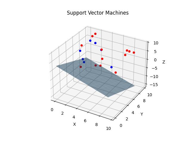
The core idea behind SVMs is to find a hyperplane that best separates the data into classes. In two dimensions, a hyperplane is just a line. In three dimensions, it is a plane, and in more than three dimensions, it becomes a hyperplane. The distance from the hyperplane to the nearest data point on either side is known as the margin. The goal of an SVM is to find the hyperplane with the largest margin.
SVM Algorithm
To understand how an SVM works, let’s consider a simple example with two classes: class A and class B. We have two-dimensional data, and we want to find the hyperplane that separates the two classes. The hyperplane can be represented as:
w1x1 + w2x2 + b = 0
Where w1 and w2 are the weights and b is the bias. The weights and bias determine the position and orientation of the hyperplane. The goal is to find the values for w1, w2, and b that best separate the two classes.
There are several ways to find the optimal hyperplane, but one common method is to use the “maximum margin” technique. The idea is to find the hyperplane that has the maximum distance from the nearest data points of both classes. This is known as the “maximum margin” hyperplane.
SVM in practice using scikit-learn
To find the maximum margin hyperplane, we need to solve a quadratic optimization problem. We can use a library such as scikit-learn in Python to solve this problem. Here’s some example code in Python using scikit-learn to train an SVM:
from sklearn import svm

# Set up the SVM model
model = svm.SVC()

# Train the model on the training data
model.fit(X_train, y_train)

# Predict on the test data
predictions = model.predict(X_test)
In this code, X_train and y_train are the training data and labels, and X_test is the test data. The fit function trains the SVM model on the training data, and the predict function predicts the labels for the test data.
One thing to note is that the SVM algorithm is sensitive to the scale of the data. It is a good practice to scale the data before training an SVM model. This can be done using the StandardScaler class from sklearn.preprocessing.
from sklearn.preprocessing import StandardScaler

# Create the scaler
scaler = StandardScaler()

# Fit the scaler to the training data
scaler.fit(X_train)

# Scale the training data
X_train_scaled = scaler.transform(X_train)

# Scale the test data
X_test_scaled = scaler.transform(X_test)

# Train the model on the scaled data
model.fit(X_train_scaled, y_train)

# Make predictions on the scaled test data
predictions = model.predict(X_test_scaled)
SVMs are a powerful and widely used method for supervised learning tasks, and they have been successful in a variety of applications including text and image classification. One advantage of SVMs is that they can perform well even with high-dimensional data, which makes them a good choice for many real-world problems.
One disadvantage of SVMs is that they can be time-consuming to train, especially for large datasets. In addition, the optimization problem that needs to be solved to find the maximum margin hyperplane is computationally expensive, which can make training SVMs impractical for very large datasets.
Another potential disadvantage of SVMs is that they can be sensitive to the choice of kernel and hyperparameters. The kernel is a function that is used to map the data into a higher-dimensional space, which can make it easier to find a hyperplane that separates the classes. Different kernels can be used, and the choice of kernel can significantly impact the performance of the SVM. In addition, there are several hyperparameters that can be adjusted, such as the regularization parameter and the kernel parameters, and finding the optimal values for these hyperparameters can be challenging.
Visualizing Results
In the example below, we use `matplotlib` to generate visualizations of the support vector machine. Although this is useful for understanding how is happening, it is only really possible in low dimensional space (ie. datasets with only a few features).
import matplotlib.pyplot as plt
from sklearn import datasets
from sklearn.svm import SVC

# Load the iris dataset as an example
iris = datasets.load_iris()
X = iris["data"][:, (2, 3)]  # petal length, petal width
y = iris["target"]

# Fit the SVM model
clf = SVC(kernel="linear")
clf.fit(X, y)

# Get the weights and bias of the decision boundary
w = clf.coef_[0]
b = clf.intercept_[0]

# Get the range of the data
x_min, x_max = X[:, 0].min() - 1, X[:, 0].max() + 1
y_min, y_max = X[:, 1].min() - 1, X[:, 1].max() + 1

# Create a grid of points to evaluate the model
xx, yy = np.meshgrid(np.arange(x_min, x_max, 0.1),
                     np.arange(y_min, y_max, 0.1))

# Get the decision boundary and margins
Z = clf.predict(np.c_[xx.ravel(), yy.ravel()])
Z = Z.reshape(xx.shape)

# Plot the data and decision boundary
plt.contourf(xx, yy, Z, cmap=plt.cm.twilight, alpha=0.8)
plt.scatter(X[:, 0], X[:, 1], c=y, cmap=plt.cm.coolwarm)
plt.plot(xx, (-w[0] * xx - b) / w[1], c="k")
plt.axis([x_min, x_max, y_min, y_max])
plt.xlabel("Petal length")
plt.ylabel("Petal width")
plt.title("SVM Decision Boundary")
plt.show()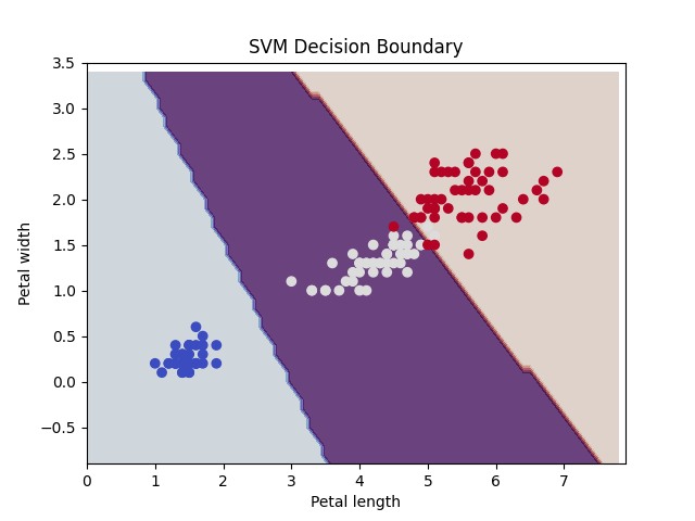
Overall, SVMs are a useful tool for many supervised learning tasks, and they can perform well with a wide range of data. With the right kernel and hyperparameter settings, they can be a powerful and effective method for classification and regression tasks.
Support vector machines (SVMs) are a popular and powerful tool for a variety of machine learning tasks. They have been used in a wide range of industries and applications, including:
- Text classification: SVMs have been used for text classification tasks such as spam detection and sentiment analysis.
- Image classification: SVMs have been used for image classification tasks such as facial recognition and object recognition.
- Bioinformatics: SVMs have been used in the field of bioinformatics for tasks such as protein classification and disease diagnosis.
- Financial forecasting: SVMs have been used in finance for tasks such as stock price prediction and credit risk assessment.
- Handwriting recognition: SVMs have been used for handwriting recognition tasks, such as reading handwritten digits or text.
- Customer segmentation: SVMs have been used in marketing to segment customers into different groups based on their characteristics and behavior.
In general, SVMs are a useful tool whenever we need to classify or predict outcomes based on labeled data. They are particularly useful in cases where the data is high-dimensional or there are a large number of features, as SVMs can handle high-dimensional data well.
In conclusion, support vector machines (SVMs) are a powerful and widely used tool for supervised learning tasks. They work by finding the hyperplane that best separates the data into classes, and they can handle high-dimensional data effectively. While they can be time-consuming to train and may be sensitive to kernel and hyperparameter choices, they have been successful in a variety of applications including text and image classification, bioinformatics, financial forecasting, handwriting recognition, and customer segmentation. With the right settings, SVMs can be a valuable tool for classification and prediction tasks.