Decision Trees

Decision trees are a popular machine learning technique for classifying data. They are simple to understand, interpret, and visualize, and they can often perform well with little hyperparameter tuning. In this article, we’ll take a look at how decision trees work and how to use them in Python.

How Decision Trees Work

Decision trees work by recursively dividing the input space into smaller and smaller regions, called “nodes,” based on the values of one or more features. At each node, the decision tree makes a decision based on the feature(s) and splits the data into two or more branches, called “children,” depending on the value of the feature(s). This process continues until the decision tree reaches a “leaf” node, which is a node that does not have any children.

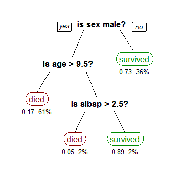
The decision tree above, for example, is used to classify whether or not a passenger on the Titanic survived. At the root node, the decision tree splits the data based on the feature “sex.” If the passenger is male, the data goes down the left branch, and if the passenger is female, the data goes down the right branch. This process continues until the data reaches a leaf node, where the decision tree makes a prediction about whether or not the passenger survived.

Decision trees are often used for classification tasks, but they can also be used for regression tasks by predicting a continuous value instead of a class.

Where are decision trees used?

Decision trees are a good choice for many classification tasks because they are simple to understand, interpret, and visualize, and they often perform well with little hyperparameter tuning. Some specific examples where decision trees might be a good choice include:

• Predicting whether a customer will churn based on their past behavior and other features.
• Predicting whether a patient has a certain disease based on their symptoms and test results.
• Predicting whether a loan application will default based on the borrower’s credit history and other factors.
• Predicting whether an email is spam based on the contents of the email and other features.
• Predicting the type of animal in an image based on the features of the image.

These are just a few examples, but decision trees can be used for many other classification tasks as well.

Choosing the Best Split

One key aspect of decision trees is choosing the best feature and value to split the data at each node. There are many ways to measure the “goodness” of a split, but one common method is to use the Gini impurity measure.

The Gini impurity measure calculates the probability of misclassifying a random element in a node.

The Gini impurity of a node is calculated as:

Where n is the number of classes and \pi is the proportion of elements in the node that belong to class i.

For example, if a node contains 50% elements of class 0 and 50% elements of class 1, the Gini impurity would be:

A node with a higher Gini impurity is less pure and therefore a worse split.

To find the best split at a node, the decision tree searches through all the features and values and selects the split that results in the lowest Gini impurity. This process is repeated at each node until the decision tree reaches a leaf node.

Building a Decision Tree in Python

Now that we’ve covered the basics of decision trees, let’s look at how to build a decision tree in Python. There are many libraries available for building decision trees in Python, but one of the most popular is scikit-learn.

To build a decision tree in scikit-learn, we’ll need to import the DecisionTreeClassifier class from the tree module:

from sklearn.tree import DecisionTreeClassifier

Next, we’ll need to prepare our data. Decision trees work with numerical data, so if our data includes categorical features, we’ll need to encode them using one-hot encoding or some other method. We’ll also need to split our data into training and test sets.

from sklearn.preprocessing import OneHotEncoder
from sklearn.model_selection import train_test_split

# Encode categorical features
one_hot_encoder = OneHotEncoder()
X = one_hot_encoder.fit_transform(X)

# Split the data into training and test sets
X_train, X_test, y_train, y_test = train_test_split(X, y, test_size=0.2)

Now that we have our data prepared, we can build our decision tree. To do this, we’ll need to instantiate a DecisionTreeClassifier object and call the fit method on our training data:

# Build the decision tree
clf = DecisionTreeClassifier()
clf.fit(X_train, y_train)

By default, the decision tree will use the Gini impurity measure to choose the best split at each node. However, we can also specify other splitting criteria, such as the information gain or the chi-squared statistic, by setting the criterion parameter.

Once the decision tree is trained, we can use it to make predictions on our test data by calling the predict method:

# Make predictions on the test set
y_pred = clf.predict(X_test)

We can then evaluate the performance of our decision tree using various metrics, such as accuracy, precision, and recall.

from sklearn.metrics import accuracy_score, precision_score, recall_score

# Calculate accuracy
accuracy = accuracy_score(y_test, y_pred)

# Calculate precision
precision = precision_score(y_test, y_pred)

# Calculate recall
recall = recall_score(y_test, y_pred)

print("Accuracy:", accuracy)
print("Precision:", precision)
print("Recall:", recall)

Tuning Decision Tree Hyperparameters

Like most machine learning models, decision trees have several hyperparameters that can be tuned to improve their performance. Some common hyperparameters to tune include:

• max_depth: The maximum depth of the tree. A higher value allows the tree to become more complex, but it can also increase the risk of overfitting.
• min_samples_split: The minimum number of samples required to split a node. A higher value can reduce the risk of overfitting, but it can also decrease the model’s ability to learn from the data.
• min_samples_leaf: The minimum number of samples required at a leaf node. A higher value can reduce the risk of overfitting, but it can also decrease the model’s ability to learn from the data.

To tune the hyperparameters of a decision tree in scikit-learn, we can use the GridSearchCV class from the model_selection module.

from sklearn.model_selection import GridSearchCV

# Define the hyperparameter grid
param_grid = {
    'max_depth: [3, 5, 7, 9],
	'min_samples_split': [2, 4, 6],
	'min_samples_leaf': [1, 3, 5]
}
# Instantiate the decision tree classifier
clf = DecisionTreeClassifier()

#Set up the grid search
grid_search = GridSearchCV(clf, param_grid, cv=5)

# Fit the grid search to the data
grid_search.fit(X_train, y_train)

#Get the best parameters
best_params = grid_search.best_params_

# Rebuild the model with the best parameters
clf = DecisionTreeClassifier(**best_params)
clf.fit(X_train, y_train)

# Make predictions on the test set
y_pred = clf.predict(X_test)

# Calculate accuracy
accuracy = accuracy_score(y_test, y_pred)

# Calculate precision
precision = precision_score(y_test, y_pred)

# Calculate recall
recall = recall_score(y_test, y_pred)

print("Accuracy:", accuracy)
print("Precision:", precision)
print("Recall:", recall)

By using the GridSearchCV class, we can try out different combinations of hyperparameters and select the ones that result in the best model performance.

Take Aways

In this article, we learned about decision trees, a popular machine learning technique for classifying data. We saw how decision trees work by recursively dividing the input space into nodes and making predictions at the leaf nodes. We also looked at how to build and tune decision trees in Python using scikit-learn. Decision trees are a simple and powerful tool for many classification tasks and are worth considering when building machine learning models.