Building a Perceptron with Python

One of the core building blocks of a neural network is the Perceptron, in this article we will be building a Perceptron with Python.

What is a perceptron?

A perceptron is one of the first computational units used in artificial intelligence. Its design was inspired by biology, the neuron in the human brain and is the most basic unit within a neural network.

A perceptron is a machine learning algorithm used within supervised learning. It’s a binary classification algorithm that makes its predictions using a linear predictor function.

For a more formal definition and history of a Perceptron see this Wikipedia article.

Perceptron use cases

Since a perceptron is a linear classifier, the most common use is to classify different types of data. In basic terms this means it can distinguish two classes within a dataset but only if those differences are linearly separable.

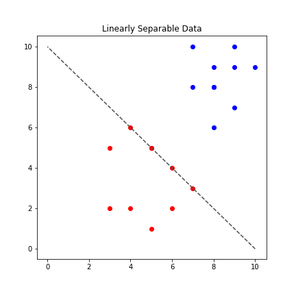
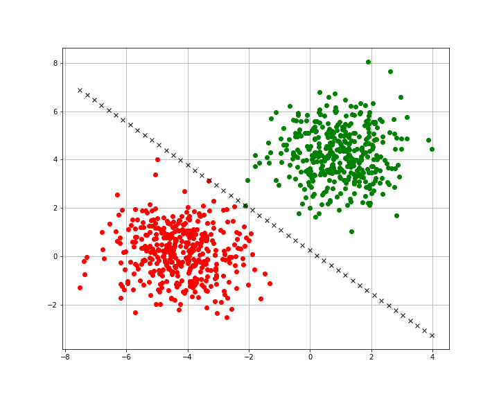
As shown in the diagram above, we can see an example of data that is linearly separable, we can draw a straight line between the red and blue dots to tell them apart.

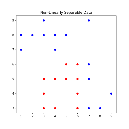
By contrast, the diagram below shows an example of a dataset that isn’t linearly separable.

Now that we understand what types of problems a Perceptron is lets get to building a perceptron with Python.

A Perceptron in Python

The perceptron algorithm has been covered by many machine learning libraries, if you are intending on using a Perceptron for a project you should use one of those.

One of the libraries I have used personally which has an optimised version of this algorithm is scikit-learn.

import matplotlib.pyplot as plt
import numpy as np
from sklearn.metrics import accuracy_score

class Perceptron(object):
    def __init__(self, lr=0.01, epochs=2000):
        self.lr = lr
        self.bias = 1
        self.epochs = epochs
        self.weights = None
        self.errors_ = []


    def fit(self, X, y):
        """Train perceptron. 
        X and y need to be the same length"""
        assert len(X) == len(y), "X and y need to be the same length"
        
        # Initialise weights
        weights = np.zeros(X.shape[1])
        self.weights = np.insert(weights, 0, self.bias, axis=0)

        for _ in range(self.epochs):
            errors = 0
            for xi, y_target in zip(X, y):
                z = self.__linear(xi)  # weighted sum
                y_hat = self.__activation(z)  # activation function
                delta = self.lr * (y_target - y_hat)  # loss
        
                # Update weights - back propagation
                self.weights[1:] += delta * xi
                self.weights[0] += delta
                
                errors += int(delta != 0.0)

            self.errors_.append(errors)          
            if not errors:
                break
    
    
    def __linear(self, X):
        """weighted sum"""
        return np.dot(X, self.weights[1:]) + self.weights[0] 

    
    def __activation(self, X):
        return np.where(X>=0, 1, 0)
                        
    
    def predict(self, X):
        assert type(self.weights) != 'NoneType', "You must run the fit method before making predictions."
        y_hat = np.zeros(X.shape[0],)
        for i, xi in enumerate(X):
            y_hat[i] = self.__activation(self.__linear(xi))
        return y_hat


    def score(sef, predictions, labels):
        return accuracy_score(labels, predictions)
    
    
    def plot(self, predictions, labels):
      	assert type(self.weights) != 'NoneType', "You must run the fit method before being able to plot results."
        plt.figure(figsize=(10,8))
        plt.grid(True)

        for input, target in zip(predictions, labels):
            plt.plot(input[0],input[1],'ro' if (target == 1.0) else 'go')

        for i in np.linspace(np.amin(predictions[:,:1]),np.amax(predictions[:,:1])):
            slope = -(self.weights[0]/self.weights[2])/(self.weights[0]/self.weights[1])  
            intercept = -self.weights[0]/self.weights[2]

            # y = mx+b, equation of a line. mx = slope, n = intercept
            y = (slope*i) + intercept
            plt.plot(i, y, color='black', marker='x', linestyle='dashed')

The algorithm (in this highly un-optimized state) isn’t that difficult to implement, but it’s important to understand the maths behind it.

Breaking down the Perceptron algorithm

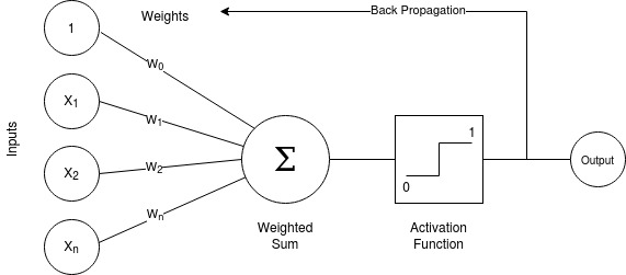
The inputs typically are referred to as X_1 \to X_n the X_0 value is reserved for the bias value and is always 1.

The 0^{th} value X_0 is set to one to ensure when we perform the weighted sum, we don’t get a zero value if one of our other weights is zero.

This value is referred to as the bias value, this is implemented here:

        self.weights = np.insert(weights, 0, self.bias, axis=0)

By inserting a 1 at the start of the array I ensure that if either of the other two values are zero, I will always get a value in the next step.

A weighted sum

Continuing on, we perform a weighted sum with all the inputs. The formula to calculate this is as follows:

\Large{\sum_{i=1}^{m} {w^{i}}{x^{i}}}

In simple terms we performing following operation:

In the perception class, this is implemented here:

    def __linear(self, X):
        """weighted sum"""
        return np.dot(X, self.weights[1:]) + self.weights[0]

Activation function

Once have the weighted sum of inputs, we put this value through an activation function.

The purpose of the activation function is to provide the actual prediction, if the value from the weighted sum is greater than 0 then the function returns a 1. Alternatively, if the value of the weighted sum is lower than zero (or negative) it returns a zero.

\normalsize{if}\Large{\sum_{i=1}^{m} {w^{i}}{x^{i}}} \normalsize{> 0} then \phi = 1

[\normalsize{if}\Large{\sum_{i=1}^{m} {w^{i}}{x^{i}}} \normalsize{< 0} then \phi = 0

The code that represents this logic can be found here:

    def __activation(self, X):
        return np.where(X>=0, 1, 0)

Back propagation – Updating weights

In terms of how the Perceptron actually learns, this is achieved with the back propagation step, also known as updating of weights.

Since we already know what the true value of the label is, we can calculate the difference between the predicted value and the actual value. This value we get from performing this calculation is know as the error.

We can then take that value an add it to our original weights in order to modify the weights. Before we perform that addition we multiply the error value by our learning rate. By doing so, we are ensuring we’re making controlled incremental adjustments to our weights.

                z = self.__linear(xi)  # weighted sum
                y_hat = self.__activation(z)  # activation function
                delta = self.lr * (y_target - y_hat)  # loss
        
                # Update weights - back propagation
                self.weights[1:] += delta * xi
                self.weights[0] += delta

Now that we can make updates to the weights we have a working perceptron. I have a couple of additional helper functions (score, plot) in the model. These functions will help with calculating accuracy as well visualizing results.

Practical Example

We have the code for a Perceptron, let’s put it to work to build a model and visualize the results.

First we need to import some additional classes from scikit-learn to assist with generating data that we can use to train our model.

from sklearn.model_selection import train_test_split
from sklearn.datasets import make_blobs

The make_blobs class will help us generate some randomised data and the train_test_split will assist with splitting our data.

A non-perfect example

In the example below we will see an instance where our data is not 100% linearly separable and how our model handles processing this dataset.

# Generate data blobs, 2 features each with two classses
X, y = make_blobs(n_samples=1000, n_features=2, centers=2, cluster_std=1.05, random_state=3)
X_train, X_test, y_train, y_test = train_test_split(X, y, test_size=0.20, stratify=y)

# Create an instance of our Perceptron
p = Perceptron()

# Fit the data, display and display our accuracy score
p.fit(X_train,y_train)
p.score(p.predict(X_test), y_test)

If you use the same random_state as I have above you will get data that’s either not completely linearly separable or some points that are very close in the middle.

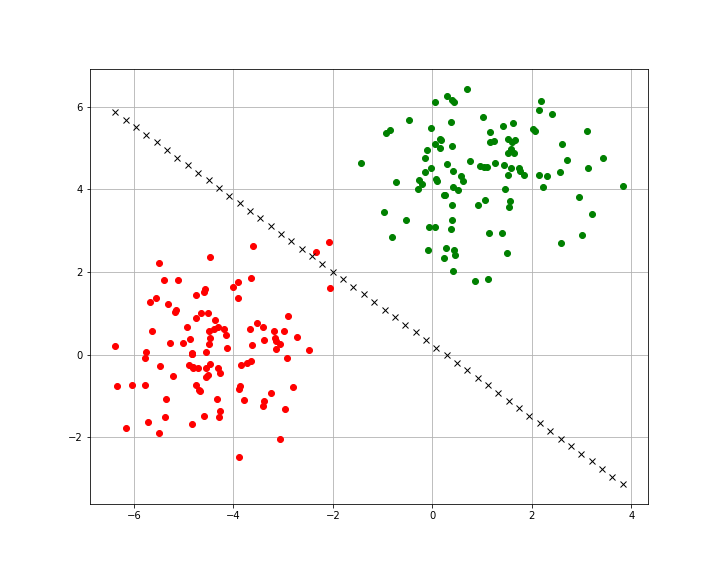
The accuracy score I got for this model was 0.99 (99% accuracy), in some cases tweaks to the learning rate or the epochs can help achieve a 100% accuracy. If we visualize the training set for this model we’ll see a similar result.

In the case of our training set, this is actually a little harder to separate. As you can see there are two points right on the decision boundary.

Feel free to try other options or perhaps your own dataset, as always I’ve put the code up on GitHub so grab a copy there and do some of your own experimentation.

If you enjoyed building a Perceptron in Python you should checkout my k-nearest neighbors article.

Complete code here – https://github.com/letsfigureout/perceptron